liquefaction modeling and 3D analysis module based on Drilling information
Development of liquefaction analysis basic data modeling and 2/3D liquefaction analysis map generation module for the efficient extraction of drilling information. The liquefaction analysis and visualization information obtained through the developed module can be used as a liquefaction damage prediction system to build a linkage and utilization system with other systems such as earthquake disaster.
1) Technology Introduction : liquefaction modeling and 3D analysis module
The liquefaction phenomenon has been officially confirmed in recent earthquakes in Pohang. Liquefaction is the phenomenon of loss of rigidity and shearing strength when the soil is stressed. In general, when liquefaction occurs, a parts of the water and sand can be ejected over the ground with creating space, so there is a risk of road erosion or sinkholes. Therefore, there is a growing need to produce a liquefaction risk maps in Korea, and this study extracts information related to national drilling information for the map and developed modules for basic data modeling and three-dimensional analysis based on the drilling information.
2) interpolation
Interpolation (or spatial interpolation) is a method of building new data points using known data points. When you need statistics on space, the best way is to acquire the data you need at every point. However, it is practically impossible to get the desired value at all points due to problems such as cost and time. Therefore, after selecting a number of specific points to obtain observation value, this value data is used to predict the value of the points to be known, and interpolation is widely used in this process. The system provides six typical interpolation methods as following.
3) Type of interpolation
A) Radial Basis Function(RBF)
It is a proposed model for the interpolation of multivariate data, so it is easy to generate compared with kriging and it expresses a system with a strong nonlinearity well, but predictive performance reacts sensitively.
B) Natural Neighbor interpolation
It is the simplest interpolation based on the Voronoi tessation of discrete spatial sets and shows relatively close approximations.
C) Inverse Distance Weight (IDW)
A method for determining the value of a new cell using linearly coupled weights from a nearby point. It is called the Inverse Distance Weight because the closer the distance is, the higher the weight is applied.
D) kriging(Triangulated Irregular Network]
It is a geo-statistical method that a linear combination of known data is used to estimate the value of the property at the point of interest. This method assumes the value by linearly combining the measured values of the surrounding with a statistical method.
When estimating the value, it reflects not only the distance from the measured value but also the correlation strength between neighboring values. It requires a large amount of calculation, but relatively accurate.
E) Triangulated Irregular Network, TIN
It is relatively suitable for small areas by connecting all points in a triangle to calculate values within the triangle.
F) Spline interpolation
Connection polynomials that gradually apply polynomials to subset of data points are called spline functions. Functions generally change smoothly, but sometimes rapidly in certain areas. Spline functions provide a good approximation to the behavior of locally and rapidly changing functions.
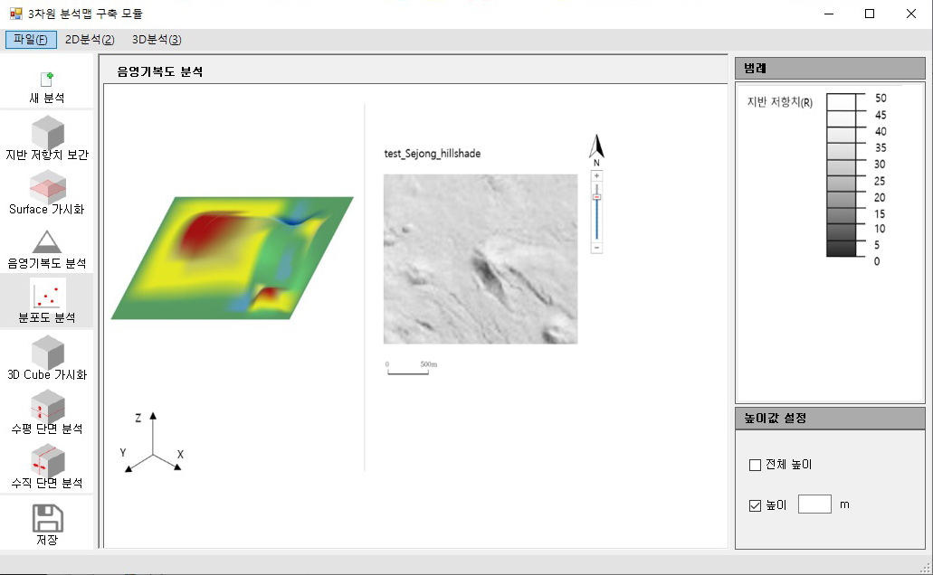
4) Visualization
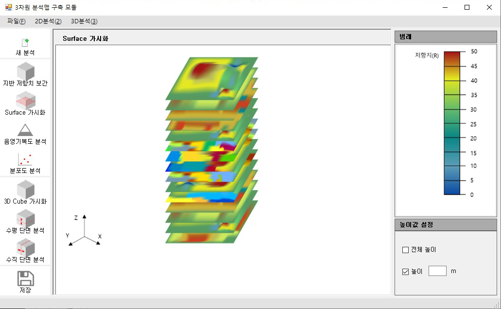
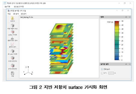
A. Surface Visualization
The surface visualization function visualizes the ground resistance value R corrected at regular intervals. When you click on the ground resistance surface visualization, the screen that the ground resistance value surface is visualized is output as shown in the picture.
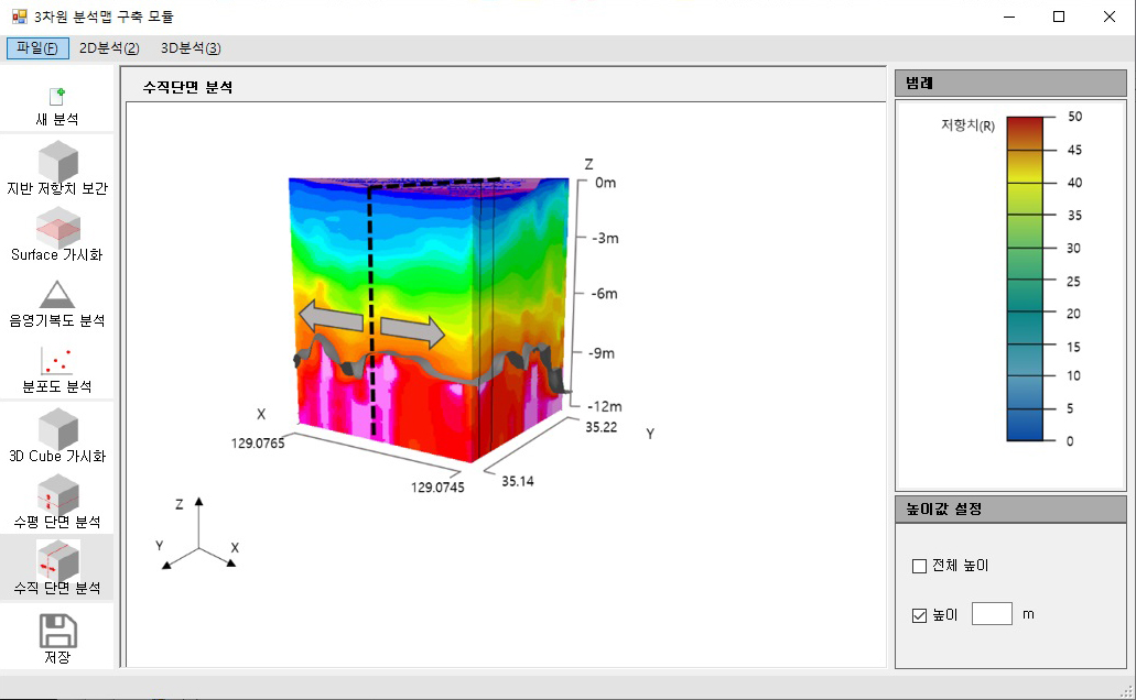
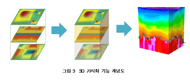
B. 3D Visualization
3D visualization is a function that makes a modeling of the 3D resistance value based on the ground resistance 2D analysis result and shows it in three dimensions. The screen shown can be enlarged/ reduced/rotated and it supports a Legend for each resistance value to help visualization. The following is a conceptual diagram that visualizes 2D analysis results in 3D cube format.